The Lagging Indicator Chronicles – A Tale of Policies Playing Catch-Up
Lag time between state-level policy interventions and change points in COVID-19 outcomes in the United States. Read more at 00149-5).
Project Overview
This project investigates the lag time between state-level policy interventions and changes in COVID-19 outcomes across the United States. Using COVID-19 confirmed cases and death data, we applied a changepoint method integrated with a random walk model with piecewise drifts to detect shifts in the growth rates of daily cases and deaths. The analysis covers data from March 2020 to February 2021.
Summary
We collected state-level daily COVID-19 confirmed cases and deaths, then cleaned and processed the data to align the timeline of the pandemic for each state. The focus was on:
- Data Preprocessing: Aligning the start date for each state’s dataset to March 5, 2020.
- Changepoint Detection: Using Genetic Algorithms (GA) to detect change points in the time series, focusing on significant changes in growth rates.
- Model Application: Applied a random walk model with piecewise drifts to model shifts in trends for each state.
- Moving Average: Implemented a 7-day moving average to smooth the data and detect significant patterns.
- Model Evaluation: Employed the Maximum Likelihood Estimation (MLE) method for fitting the model and assessing its performance.
Walk-Through
Data Preprocessing
The dataset spans from March 2020 to February 2021 and contains state-level records of daily COVID-19 cases and deaths. The first step was to ensure the timelines across all states aligned by setting a uniform start date. Data for each state was extracted and trimmed to fit the analysis period.


Changepoint Detection Using GA
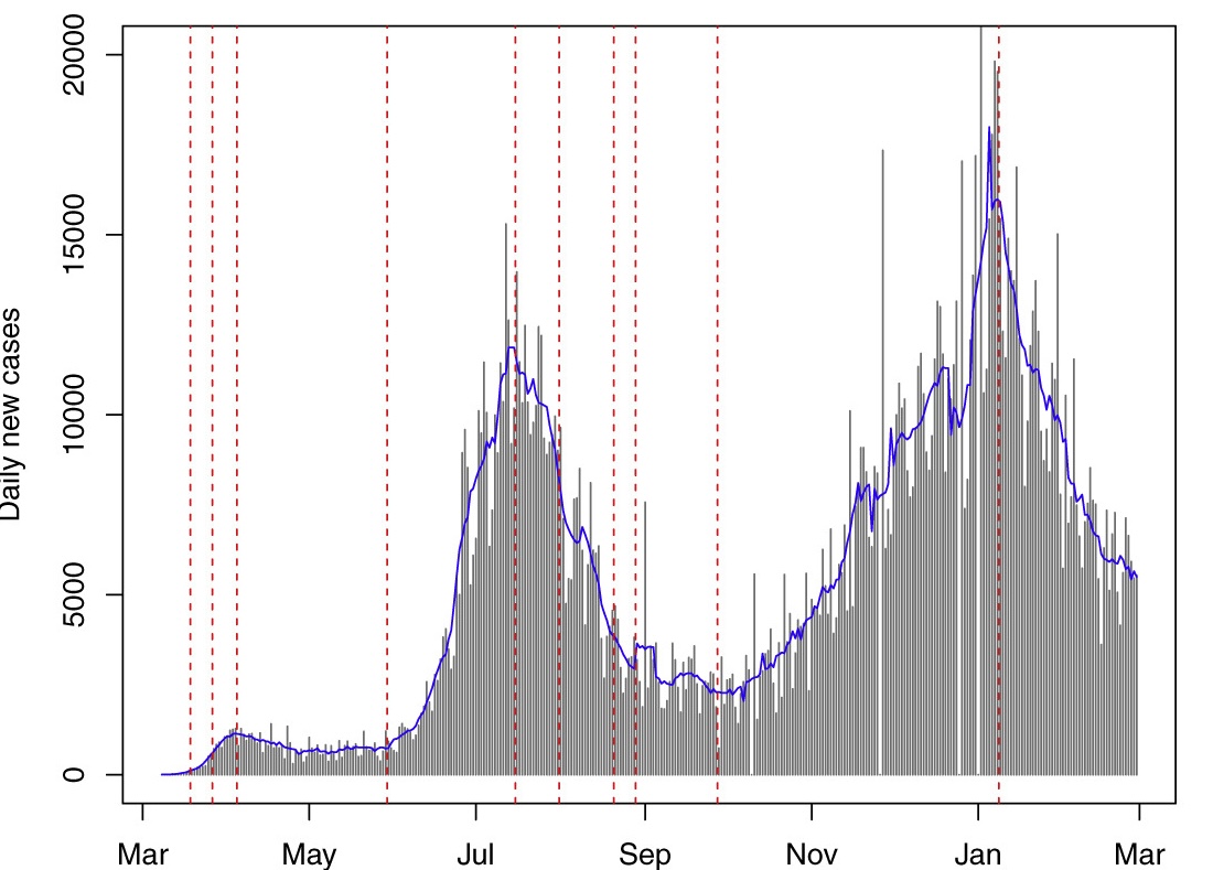
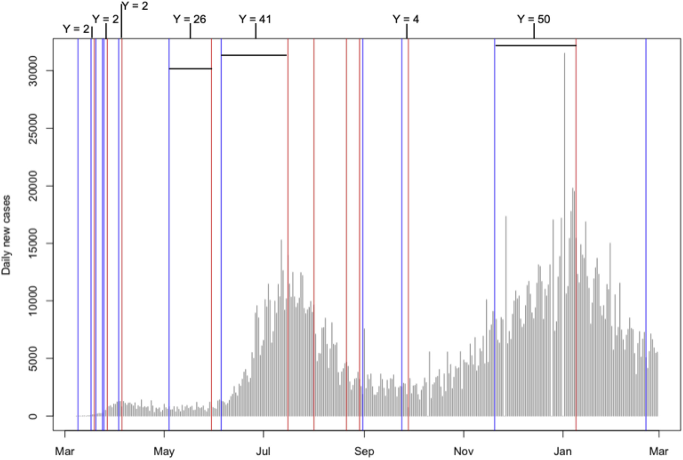
To detect change points, we implemented a Genetic Algorithm (GA). The GA scans through the dataset to identify significant changes in the rate of COVID-19 spread within each state. The primary goal was to highlight points in time where policy interventions led to a measurable impact on the case and death growth rates.
Random Walk Model with Piecewise Drifts
A random walk model with piecewise drifts was applied to each state’s time series data. The model divides the time series into segments where the drift (trend) changes at each detected changepoint. By modeling the drift changes, we aimed to capture the effects of policy interventions at various stages of the pandemic.
Moving Average and Smoothing
To reduce noise in the data, we applied a 7-day moving average. This smoothed out day-to-day fluctuations and allowed for a clearer view of trends and shifts in COVID-19 outcomes.
Model Evaluation and Results
Once changepoints were detected, the Maximum Likelihood Estimation (MLE) method was used to fit the random walk model to the data. The model was evaluated based on its ability to accurately detect changes in the spread of COVID-19 following policy interventions.
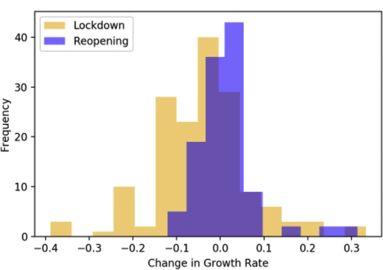
The analysis revealed significant lag times between policy implementations and the resulting change points in case and death growth rates. This information can be useful for future public health responses.
We consider the following random walk model with stepwise drifts:
\[\ln X_t = \ln X_{t-1} + \Delta_t + Z_t\]where:
- \(X_t\) is the 7-day moving average of the COVID-19 outcome (either confirmed cases or deaths) on day \(t\),
- \(\Delta_t\) is a time-dependent stepwise drift that changes at unknown change points \(\tau_1, \tau_2, \dots, \tau_m\),
- \(Z_t \sim N(0, \omega^2)\) is Gaussian white noise with variance \(\omega^2\).
Model Parameters
The stepwise drift \(\Delta_t\) is defined as:
\[\Delta_t = \begin{cases} \delta_1 & 1 \leq t < \tau_1 \\ \delta_2 & \tau_1 \leq t < \tau_2 \\ \vdots & \vdots \\ \delta_{m+1} & \tau_m \leq t \leq n \end{cases}\]Here, \(m\) is the number of change points, and \(\delta_j\) is the drift in regime \(j\).
Likelihood Function
Given the model, the difference in log-transformed outcomes is:
\[\ln X_t - \ln X_{t-1} = \Delta_t + Z_t\]We assume that \(Z_t \sim N(0, \omega^2)\). Thus, for each regime \(j\), we have:
\[\ln X_t - \ln X_{t-1} \sim N(\delta_j, \omega_j^2)\]The log-likelihood for observations \(X_1, X_2, \dots, X_n\) given the parameters \(\{\delta_j, \omega_j^2\}\) and change points \(\{\tau_j\}\) is:
\[\mathcal{L}(\delta, \omega^2; X_1, \dots, X_n) = -\frac{1}{2} \sum_{j=1}^{m+1} \sum_{t=\tau_{j-1}}^{\tau_j-1} \left[ \ln(2\pi \omega_j^2) + \frac{(\ln X_t - \ln X_{t-1} - \delta_j)^2}{\omega_j^2} \right]\]where \(\tau_0 = 1\) and \(\tau_{m+1} = n+1\).
To find the MLE of \(\delta_j\) and \(\omega_j^2\), we differentiate the log-likelihood with respect to \(\delta_j\) and \(\omega_j^2\) and set the derivatives to zero.
The MLE for \(\delta_j\) is obtained by solving:
\[\frac{\partial \mathcal{L}}{\partial \delta_j} = 0\]This gives:
\[\hat{\delta}_j = \frac{1}{n_j} \sum_{t=\tau_{j-1}}^{\tau_j-1} (\ln X_t - \ln X_{t-1})\]where \(n_j = \tau_j - \tau_{j-1}\) is the number of observations in regime \(j\).
The MLE for \(\omega_j^2\) is obtained by solving:
\[\frac{\partial \mathcal{L}}{\partial \omega_j^2} = 0\]This gives:
\[\hat{\omega}_j^2 = \frac{1}{n_j} \sum_{t=\tau_{j-1}}^{\tau_j-1} (\ln X_t - \ln X_{t-1} - \hat{\delta}_j)^2\]Conclusion
This project provides a comprehensive analysis of the lag times between state-level policy interventions and their effects on COVID-19 outcomes. By combining changepoint detection using Genetic Algorithms and a random walk model, we were able to capture the dynamic nature of the pandemic’s progression across the United States.
The results offer insights that can aid in decision-making for public health policies in response to similar crises.